
Broadly, statistics is concerned with collecting and analyzing data. It seeks to describe rigorous methods for collecting data (samples), for describing the data, and for inferring conclusions from the data. There are processes out there in the world that generate observable data, but these processes are often black boxes and we want to gain some insight into how they work.
We can crudely cleave statistics into two main practices: descriptive statistics, which provides tools for describing data, and inferential statistics, which provides tools for learning (inferring or estimating) from data.
This section is focused on frequentist (or classical) statistics, which is distinguished from Bayesian statistics (covered in another chapter).
Descriptive statistics involves computing values which summarize a set of data. This typically includes statistics like the mean, standard deviation, median, min, max, etc, which are called summary statistics.
In statistics, numbers and variables are categorized in certain ways.
Variables may be categorical (also called qualitative), in which they represent discrete values (numbers here are arbitrarily assigned to represent categories of qualities), or numerical (also called quantitative) in which they represent continuous values.
These variables are further categorized into scales of measurement.
The average of a set of data can be described as its central tendency; which gives some sense of a typical or common value for a variable. There are three types:
Often just called the "mean" and notated
For a dataset
The mean can be sensitive to extreme values (outliers), which is one reason the median is sometimes used instead. Which is to say, the median is a more robust statistic (meaning that it is less sensitive to outliers).
Note that there are other types of means, but the arithmetic mean is by far the most common.
The central value in the dataset, e.g.
If there are even number of values, you just take the value between the two central values:
The most frequently occurring value in the dataset, e.g.
With statistics we take a sample of a broader population or already have data which is a sample from a population. We use this limited sample in order to learn things about the whole population.
The mean of the population is denoted
The sample mean is:
The sample variance is:
The sample covariance matrix is:
These estimators are unbiased, i.e.:
Often in statistics we assume that a sample is independent and identically distributed (iid); that is; that the data points are independent from one another (the outcome of one has no influence over the outcome of any of the others) and that they share the same distribution.
We say that
In this case, they all share the same mean (expected value) and variance.
This assumption makes computing statistics for the sample much easier.
For instance, if a sample was not identically distributed, each datapoint might come from a different distribution, in which case there are different means and variances for each datapoint which must be computed from each of those datapoints alone. They can't really be treated as a group since the datapoints aren't quite equivalent to each other (in a statistical sense).
Or, if the sample was not independent, then we lose all the conveniences that come with independence.
The IID assumption doesn't always hold (i.e. it may be violated), of course, so there are other ways of approaching such situations while minimizing complexity, such as Hidden Markov Models.
Let
The law of large numbers essentially states that as a sample size approaches infinity, its mean will approach the population ("true") mean:
Say you have a set of data. Even if the distribution of that data is not normal, you can divide the data into groups (samples) and then average the values of those groups. Those averages will approach the form of a normal curve as you increase the size of those groups (i.e. increase the sample size).
Let
Then the central limit theorem can be formalized as:
That is, the left side converges in distribution to a normal distribution with mean 0 and variance 1 as
Dispersion is the "spread" of a distribution - how spread it out its values are.
The main measures of dispersion are the variance and the standard deviation.
Standard deviation is represented by
The square of the standard deviation, that is,
For a population of size
That is, variance is the difference between the square of the inputs and the square of the expected value.
Variance depends on the units of measurement, but this can be controlled for by computing the coefficient of variation:
This allows us to compare variability across variables measured in different units.
The variance of a linear combination of (independent) random variables, e.g.
The range can also be used to get a sense of dispersion. The range is the difference between the highest and lowest values, but very sensitive to outliers.
As an alternative to the range, you can look at the interquartile range, which is the range of the middle 50% of the values (that is, the difference of the 75th and 25th percentile values). This is less sensitive to outliers.
A Z score is just the number of standard deviations a value is from the mean. It is defined:
The empirical rule describes that, for a normal distribution, there is:

If you have reason to expect that the standard deviations of two populations are practically identical, you can use the pooled standard deviation of the two groups to obtain a more accurate estimate of the standard deviation and standard error:
Where
The
The
The third moment is the skewness, and the fourth moment is the kurtosis; they all share the same form (with different normalization terms):
Moments have different units, e.g. the first moment might be in meters (
The covariance describes the variance between two random variables.
For random variables
There must the same number of values
This is simplified to:
A positive covariance means that as
A negative covariance means that as
Note that variance is just the covariance of a random variable with itself:
Correlation gives us a measure of relatedness between two variables. Alone it does not imply causation, but it can help guide more formal inquiries (e.g. experiments) into causal relationships.
A good way to visually intuit correlation is through scatterplots.
We can measure correlation with correlation coefficients. These measure the strength and sign of a relationship (but not the slope, linear regression, detailed later, does that).
Some of the more common correlation coefficients include:
The Pearson and Spearman coefficients are the most commonly used ones, but sometimes the later two are used in special cases (e.g. with categorical data).
Note: this is sometimes denoted as a capital
You may recognize this as:
Here we convert our values to standard scores, i.e.
For a population,
This value can range from
To test the statistical significance of the Pearson correlation coefficient, you can use the
For instance, if you believe there is a relationship between two variables, you set your null hypothesis as
Then look up the value in a
The Pearson correlation coefficient tells you the strength and direction of a relationship, but it doesn't tell you how much variance of one variable is explained by the other.
For that, you can use the coefficient of determination which is just
Note that Pearson's correlation only accurately measures linear relationships; so even if you have a Pearson correlation near 0, it is still possible that there may be a strong nonlinear relationship. It's worthwhile to look at a scatter plot to verify.
It is also not robust in the presence of outliers.
Here you compute ranks (i.e. the indices in the sorted sample) rather than standard scores.
For example, for the dataset
Then you can compute the Spearman correlation:
Where
Generally, you can interpret
You can test its statistical significance using a
Spearman's correlation is more robust to outliers and skewed distributions.
This correlation coefficient is useful when comparing a categorical (binary) variable with an interval or ratio scale variable:
Where
This allows you to measure the correlation between two categorical (binary) variables.
It is calculated like so:
Where
Degrees of freedom describes the number of variables that are "free" in what value they can take. Often a given variable must be a particular value because of the values the other variables take on and some constraint(s).
For example: say we have four unknown quantities
Often data has a temporal component; e.g. you are looking for patterns over time.
Generally, time series data may have the following parts: a trend, which is some function reflecting persistent changes, seasonality; that is, periodic variation, and of course there is going to be some noise - random variation - as well.
To extract a trend from a series, you can use regression, but sometimes you will be better off with some kind of moving average. This divides the series into overlapping regions, windows, of some size, and takes the averages of each window. The rolling mean just takes the mean of each window. There is also the exponentially-weighted moving average (EWMA) which gives a weighted average, such that more recent values have the highest weight, and values before that have weights which drop off exponentially. The EWMA takes an additional span parameter which determines how fast the weights drop off.
In time series data you may expect to see patterns. For example, if a value is low, it may stay low for a bit, if it's high, it may stay high for a bit. These types of patterns are serial correlations, also called autocorrelation (so-called because it is correlated a dataset with itself, in some sense), because the values correlate in their sequence.
You can compute serial correlation by shifting the time series by some interval, called a lag, and then compute the correlation of the shifted series with the original, unshifted series.
Survival analysis describes how long something lasts. It can refer to the survival of, for instance, a person - in the context of disease, a 5-year survival rate is the probability of surviving 5 years after diagnosis, for example - or a mechanical component, and so on. More broadly it can be seen as looking at how long something lasts until something happens - for instance, how long until someone gets married.
A survival curve is a function
The survival curve ends up just being the complement of the CDF:
Looking at it this way, the CDF is the probability of a lifetime less than or equal to
A hazard function tells you the fraction of cases that continue until
Hazard functions are also used for estimating survival curves.
Often we do not have the CDF of lifetimes so we can't easily compute the survival curve. We often have non-survival cases alongside have survival cases, where we don't yet know what their final lifetime will be. Often, as is the case in the medical context, we don't want to wait to learn what these unknown lifetimes will be. So we need to estimate the survival curve with the data we do have.
The Kaplan-Meier estimation allows us to do this. We can use the data we have to estimate the hazard function, and then convert that into a survival curve.
We can convert a hazard function into an estimate of the survival curve, where each point at time
Statistical inference is the practice of using statistics to infer some conclusion about a population based on only a sample of that population. This can be the population's distribution - we want to infer from the sample data what the "true" distribution (the population distribution) is and the unknown parameters that define it.
Generally, data is generated by some process; this data-generating process is also noisy; that is, there is a relatively small degree of imprecision or fluctuation in values due to randomness. In inferential statistics, we try to uncover the particular function that describes this process as closely as possible. We do so by choosing a model (e.g. if we believe it can be modeled linearly, we might choose linear regression, otherwise we might choose a different kind of model such as a probability distribution; modeling is covered in greater detail in the machine learning part). Once we have chosen the model, then we need to determine the parameters (linear coefficients, for example, or mean and variance for a probability distribution) for that model.
Broadly, the two paradigms of inference are frequentist, which relies on long-run repetitions of an event, that is, it is empirical (and could be termed the "conventional" or "traditional" framework, though there's a lot of focus on Bayesian inference now) and Bayesian, which is about generating a hypothesis distribution (the prior) and updating it as more evidence is acquired. Bayesian inference is valuable because there are many events which we cannot repeat, but we still want to learn something about.
The frequentist believes these unknown parameters have precise "true" values which can be (approximately) uncovered. In frequentist statistics, we can estimate these exact values. When we estimate a single value for an unknown, that estimation is called a point estimate. This is in contrast to describing a value estimate as a probability distribution, which is the Bayesian method. The Bayesian believes that we cannot express these parameters as single values and we should rather describe them as a distributions of possible values to be explicit about their uncertainty.
Here we focus on frequentist inference; Bayesian inference is covered in a later chapter.
In frequentist statistics, the factor of noise means that we may see relationships (and thus come up with non-zero parameters) where they don't exist, just because of the random noise. This is what p-values are meant to compensate for - if the relationship truly did not exist, what's the probability, given the data, that we'd see the non-zero parameter estimate that we computed? Generally if this probability is less than 0.05 (i.e.
Often with statistical inference you are trying to quantify some difference between groups (which can be framed as measuring an effect size) or testing if some data supports or refutes some hypothesis, and then trying to determine whether or not this difference or effect can be attributed to chance (this is covered in the section on experimental statistics).
A word of caution: many statistical tools work only under certain conditions, e.g. assumptions of independence, or for a particular distribution, or a large enough sample size, or lack of skew, and so on - so before applying statistical methods and drawing conclusions, make sure the tools are appropriate for the data. And of course you must always be cautious of potential biases involved in the data collection process.
Dealing with error is a big part of statistics and some error is unavoidable (noise is natural).
There are three kinds of error:
We never know the true value of something, only what we observe by imprecise means, so we always must grapple with error.
We can think of the population as representing the underlying data generating process and consider these parameters as functions of the population. To estimate these parameters from the sample data, we use estimators, which are functions of the sample data that return an estimate for some unknown value. Essentially, any statistic is an estimator. For instance, we may estimate the population mean by using the sample mean as our estimator. Or we may estimate the population variance as the sample variance. And so on.
Estimators may be biased for small sample sizes; that is, it tends to have more error for small sample sizes.
Say we are estimating a parameter
Where
There are unbiased estimators as well, which have an expected mean error (against the population parameter) of 0. That is,
For example, an unbiased estimator for population variance
An estimator may be asymptotically unbiased if
Generally, unbiased estimators are preferred, but sometimes biased estimators have other properties which make them useful.
For an estimate, we can measure its standard error (SE), which describes how much we expect the estimate to be off by, on average. It can also be stated as:
"Standard error" sometimes refers to the standard error of the mean, which is the standard deviation of the mean:
Much of statistical inference is concerned with measuring the quality of these estimates.
When we used a biased estimator, we generally still want our point estimates to converge to the true value of the parameter. This property is called consistency. For some error
Given an unknown population parameter, we may want to estimate a single value for it - this estimate is called a point estimate. Ideally, the estimate is as close to the true value as possible.
The estimation formula (the function which yields an estimate) is called an estimator and is a random variable (so there is some underlying distribution). A particular value of the estimator is the estimate.
A simple example: we have a series of trials with some number of successes. We want an estimate for the probability of success of the event we looked at. Here an obvious estimate is be the number of successes over the total number of trials, so our estimator would be
We consider a "good" estimator one whose distribution is concentrated as closely as possible around the parameter's true value (that is, it has a small variance). Generally this becomes the case as more data is collected.
We can take multiple samples (of a fixed size) from a population and compute a point estimate (e.g. for the mean) from each. Then we can consider the distribution of these point estimates - this distribution is called a sampling distribution. The standard deviation of the sampling distribution describes the typical error of a point estimate, so this standard deviation is known as the standard error (SE) of the estimate.
Alternatively, if you have only one sample, the standard error of the sample mean
This however requires the population standard deviation,
Also remember that the distribution of sample means approximates a normal distribution, with better approximation as sample size increases, as described by the central limit theorem. Some other point estimates' sampling distribution also approximate a normal distribution. Such point estimates are called normal point estimates.
There are other such computations for the standard error of other estimates as well.
We say a point estimate is unbiased if the sampling distribution of the estimate is centered at the parameter it estimates.
Nuisance parameters are values we are not directly interested in, but still need to be dealt with in order to get at what we are interested in.
Rather than provide a single value estimate of a population parameter, that is, a point estimate, it can be better to provide a range of values for the estimate instead. This range of values is a confidence interval. The confidence interval is the range of values where an estimate is likely to fall with some percent probability.
Confidence intervals are expressed in percentages, e.g. the "95% confidence interval", which describes the plausibility that the parameter is in that interval. It does not imply a probability (that is, it does not mean that the true parameter has a 95% chance of being in that interval), however. Rather, the 95% confidence interval is the range of values in which, over repeated experimentation, in 95% of the experiments, that confidence interval will contain the true value. To put it another way, for the 95% confidence interval, out of every 100 experiments, at least 95 of their confidence intervals will contain the true parameter value. You would say "We are 95% confident the population parameter is in this interval".
Confidence intervals are a tool for frequentist statistics, and in frequentist statistics, unknown parameters are considered fixed (we don't express them in terms of probability as we do in Bayesian statistics). So we do not associate a probability with the parameter. Rather, the confidence interval itself is the random variable, not the parameter. To put it another way, we are saying that 95% of the intervals we would generate from repeated experimentation would contain the real parameter - but we aren't saying anything about the parameter's value changing, just that the intervals will vary across experiments.
The mathematical definition of the 95% confidence interval is (where
Where
We can compute the 95% confidence interval by taking the point estimate (which is the best estimate for the value) and
For the confidence interval of the mean, we can be more precise and look within
Sometimes we don't want the parameters of our data's distribution, but just a smoothed representation of it. Kernel density estimation allows us to get this representation. It is a nonparametric method because it makes no assumptions about the form of the underlying distribution (i.e. no assumptions about its parameters).

Some kernel function (which generates symmetric densities) is applied to each data point, then the density estimate is formed by summing the densities. The kernel function determines the shape of these densities and the bandwidth parameter,

In this figure, the grey curve is the true density, the red curve is the KDE with
Experimental statistics is concerned with hypothesis testing, where you have a hypothesis and want to learn if your data supports it. That is, you have some sample data and an apparent effect, and you want to know if there is any reason to believe that the effect is genuine and not just by chance.
Often you are comparing two or more groups; more specifically, you are typically comparing statistics across these groups, such as their means. For example, you want to see if the difference of their means is statistically significant; which is to say, likely that it is a real effect and not just chance.
The "classical" approach to hypothesis testing, null hypothesis significance testing (NHST), follows this general structure:
Broadly speaking, there are two types of scientific studies: observational and experimental.
In observational studies, the research cannot interfere while recording data; as the name implies, the involvement is merely as an observer.
Experimental studies, however, are deliberately structured and executed. They must be designed to minimize error, both at a low level (e.g. imprecise instruments or measurements) and at a high-level (e.g. researcher biases).
The power of a study is the likelihood that it will distinguish an effect of a certain size from pure luck. - Statistical power and underpowered statistics, Alex Reinhart
Statistical power, sometimes called sensitivity, can be defined as the probability of rejecting the null hypothesis when it is false.
If
Power...
Bias can enter studies primarily in two ways:
To prevent selection bias (selecting samples in such a way that it encourages a particular outcome, whether done consciously or not), sample selection may be random.
In the case of medical trials and similar studies, random allocation is ideally double blind, so that neither the patient nor the researchers know which treatment a patient is receiving.
Another sample selection technique is stratified sampling, in which the population is divided into categories (e.g. male and female) and samples are selected from those subgroups. If the variable used for stratification is strongly related to the variable being studied, there may be better accuracy from the sample size.
You need large sample sizes because with small sample sizes, you're more sensitive to the effects of chance. e.g. if I flip a coin 10 times, it's feasible that I get heads 6/10 times (60% of the time). With that result I couldn't conclusively say whether or not that coin is rigged. If I flip that coin 1000 times, it's extremely unlikely that I will get heads 60% of the time (600/1000 times) if it were a fair coin.
Sometimes to increase sample size, a researcher may use a technique called "replication", which is simply repeating the measurements with new samples. but some researchers really only "pseudoreplicate". samples should be as independent from each other as possible - otherwise you have too many confounding factors. in medical research, researchers may sample a single patient multiple times, every week for instance, and treat each week's sample as a distinct sample. this is pseudoreplication - you begin to inflate other factors particular to that patient in your results. another example is - say you wanted to measure pH levels in soil samples across the US. well, you cant sample soil 15ft from each other because they are too dependent on each other:
Operationalization is the practice of coming up with some way of measuring something which cannot be directly measured, such as intelligence. This may be accomplished via proxy measurements.
In an experiment, the null hypothesis, notated
When running an experiment, you do it under the assumption that the null hypothesis is true. Then you ask: what's the probability of getting the results you got, assuming the null hypothesis is true? If that probability is very small, the null hypothesis is likely false. This probability - of getting your results if the null hypothesis were true - is called the P value.
A type 1 error is one where the null hypothesis is rejected, even though it is true.
Type 1 errors are usually presented as a probability of them occurring, e.g. a "0.5% chance of a type 1 error" or a "type 1 error with probability of 0.01".
P values are central to null hypothesis significance testing (NHST), but they are commonly misunderstood.
P values do not:
There's no mathematical tool to tell you if your hypothesis is true; you can only see whether it is consistent with the data, and if the data is sparse or unclear, your conclusions are uncertain. - Statistics Done Wrong, Alex Reinhart
So what is it then? The P value is the probability of seeing your results or data if the null hypothesis were true.
That is, given data
If instead we want to find the probability of our hypothesis given the data, that is,
Note that P values are problematic when testing multiple hypotheses (multiple testing or multiple comparisons) because any "significant" results (as determined by P value comparisons, e.g.
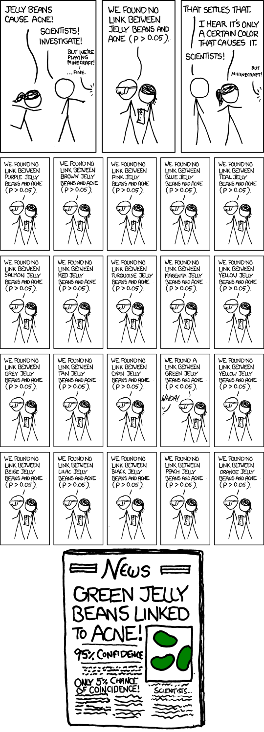
In this comic, 20 hypotheses are tested, so with a significance level at 5%, it's expected that at least one of those tests will come out significant by chance. In the real world this may be problematic in that multiple research groups may be testing the same hypothesis and chances may be such that one of them gets significant results.
A very important shortcoming to be aware of is the base rate fallacy. A P value cannot be considered in isolation. The base rate of whatever occurrence you are looking at must also be taken into account. Say you are testing 100 treatments for a disease, and it's a very difficult disease to treat, so there's a low chance (say 1%) that a treatment will actually be successful. This is your base rate. A low base rate means a higher probability of false positives - treatments which, during the course of your testing, may appear to be successful but are in reality not (i.e. their success was a fluke). A good example is the mammogram test example (see The p value and the base rate fallacy).
A p value is calculated under the assumption that the medication does not work and tells us the probability of obtaining the data we did, or data more extreme than it. It does not tell us the chance the medication is effective. (The p value and the base rate fallacy, Alex Reinhart)
The false discovery rate is the expected proportion of false positives (Type 1 errors) amongst hypothesis tests.
For example, if we have a maximum FDR of 0.10 and we have 1000 observations which seem to indicate a significant hypothesis, then we can expect 100 of those observations to be false positives.
The q value for an individual hypothesis is the minimum FDR at which the test may be called significant.
Say you run multiple comparisons and have the following values:
We can calculate the FDR as:
Note that
The value that you select to compare the p-value to, e.g. 0.5 in the comic, is the alpha level
There are some approaches to help adjust the alpha level.
The highly conservative Bonferroni Correction can be used as a safeguard.
You divide whatever your significance level
A more sensitive correction, the Sidak Correction, can also be used:
For
For
Approaches like the Bonferroni correction lowers the alpha level which end up decreasing your statistical power - that is, you fail to detect false effects as well as true effects.
And with such an approach, you are still susceptible to the base rate fallacy, and may still have false positives. So how can you calculate the false discovery rate? That is, what fraction of the statistically Significant results are false positives?
You can use the Benjamini-Hochberg procedure, which tells you which P values to consider statistically significant:
The procedure guarantees that out of all statistically significant results, no more than q percent will be false positives.
The Benjamini-Hochberg procedure is fast and effective, and it has been widely adopted by statisticians and scientists in certain fields. It usually provides better statistical power than the Bonferroni correction and friends while giving more intuitive results. It can be applied in many different situations, and variations on the procedure provide better statistical power when testing certain kinds of data.
Of course, it's not perfect. In certain strange situations, the Benjamini-Hochberg procedure gives silly results, and it has been mathematically shown that it is always possible to beat it in controlling the false discovery rate. But it's a start, and it's much better than nothing. - (Controlling the false discovery rate, Alex Reinhart)
Asks "What is the chance of seeing an effect as big as the observed effect, without regard to its sign?" That is, you are looking for any effect, increase or decrease.
Asks "What is the chance of seeing an effect as big as the observed effect, with the same sign?" That is, you are looking for either only an increase or decrease.
The most basic statistical test, used when comparing the means from two groups. Used for small sample sizes. The t-test returns a p-value.
The paired t-test is a t-test used when each datapoint in one group corresponds to one datapoint in the other group.
When comparing proportions of two populations, it is common to use the chi-squared statistic:
Where
Say for example you want to test if a coin is fair. You expect that, if it is fair, you should see about 50/50 heads and tails - this describes your expected frequencies. You flip the coin and observe the actual resulting frequencies - these are your observed frequencies.
The Chi squared test allows you to determine if these frequencies differ significantly.
ANOVA, ANCOVA, MANOVA, and MANCOVA are various ways of comparing different groups.
ANOVA is used to compare three or more groups. It uses a single test to compare the means across multiple groups simultaneously, which avoids using multiple tests to make multiple comparisons (which can lead to differences across groups resulting from chance).
There are a few requirements:
ANOVA tests the null hypothesis that the means across groups are the same (that is, that
The MSG is calculated:
Where the SSG is the sum of squares between groups and
We need a value to compare the MSG to, which is the mean square error (MSE), which measures the variability within groups and has degrees of freedom
The MSE is calculated:
Where the SSE is the sum of squared errors and is computed as:
Where the SSG is same as before and the SST is the sum of squares total:
ANOVA uses a test statistic called
When the null hypothesis is true, difference in variability across sample means should be due only to chance, so we expect MSG and MSE to be about equal (and thus
We take this
Similar to a t-test but used to compare three or more groups. With ANOVA, you calculate the F statistic, assuming the null hypothesis^[Remember that
Allows you to compare the means of two or more groups when there are multiple variables or factors to be considered.
In a two-tailed test, both tails of a distribution are considered. For example, with a drug where you're looking for any effect, positive or negative.
In a one-tailed, only one tail is considered. For example, you may be looking only for a positive or only for a negative effect.
A big part of statistical inference is measuring effect size, which more generally is trying to quantify differences between groups, but typically just referred to as "effect size".
There are a few ways of measuring effect size:
The difference in means, e.g.
But this has a few problems:
The overlap between the two distributions:
Choose some threshold between the two means, e.g.
Count how many in the first group are below the threshold, call it
Count how many in the second group are above the threshold, call it
The overlap then is:
Where
This overlap can also be framed as a misclassification rate, which is just
These measures are unitless, which makes them easy to compare across studies.
The "probability of superiority" is the probability that a randomly chosen datapoint from group 1 is greater than a randomly chosen datapoint from group 2.
This measure is also unitless.
Cohen's
This measure is also unitless.
Different fields have different intuitions about how big a
Reliability refers to how consistent or repeatable a measurement is (for continuous data).
There are three main approaches:
Aka test-retest reliability. This is how a test holds up over repeated testing, e.g. "temporal stability". This assumes the underlying metric does not change.
Aka parallel-forms reliability. This asks: how consistent are different tests at measuring the same thing?
This asks: do the items on a test all measure the same thing?
Agreement is similar to reliability, but used more for discrete data.
Note that a high percent agreement may be obtained by chance.
Often just called kappa, this corrects for the possibility of chance agreement:
Where
Occasionally you may find data easier to work with if you apply a transformation to it; that is, rescale it in some way. For instance, you might take the natural log of your values, or the square root, or the inverse. This can reduce skew and the effect of outliers or make linear modeling easier.
The function which applies this transformation is called a link function.
Data can be missing for a few reasons:
There are a few strategies for dealing with missing data.
The worst you can do is to ignore the missing data and try to run your analysis, missing data and all (it likely won't and probably shouldn't work).
Alternatively, you can delete all datapoints which have missing data, leaving only complete data points - this is called complete case analysis. Complete case analysis makes the most sense with MCAR missing data - you will have a reduction in sample size, and thus a reduction in statistical power, as a result, but your inference will not be biased. The possibly systemic nature of missing data in MAR and MNAR means that complete case analysis may overlook important details for your model.
You also have the option of filling in missing values - this is called imputation (you "impute" the missing values). You can, for instance, filling in missing values with the mean of that variable. You don't gain any of the information that was missing, and you end up ignoring the uncertainty associated with the fill-in value (and the resulting variances will be artificially reduced), but you at least get to maintain your sample size. Again, bias may be introduced in MAR and MNAR situations since the missing data may be due to some systemic cause.
One of the better approaches is multiple imputation, which produces unbiased parameter estimates and accounts for the uncertainty of imputed values. A regression model is used to generated the imputed values, and does well especially under MAR conditions - the regression model may be able to exploit info in the dataset about the missing data. If some known values correlate with the missing values, they can be of use in this way.
Then, instead of using the regression model to produce one value for each missing value, multiple values are produced, so that the end result is multiple copies of your dataset, each with different imputed values for the missing values. Your perform your analysis across all datasets and average the produced estimates.
Resampling involves repeatedly drawing subsamples from an existing sample.
Resampling is useful for assessing and selecting models and for estimating the precision of parameter estimates.
A common resampling method is bootstrapping.
Bootstrapping is a resampling method to approximate the true sampling distribution of a dataset, which can then be used to estimate the mean and the variance of the distribution. The advantage with bootstrapping is that there is no need to compute derivatives or make assumptions about the distribution's form.
You take
Then you can estimate the mean and variance:
With bootstrap estimates, there are two possible sources of error. You may have the sampling error from your original sample