
In supervised learning, the learning algorithm is provided some pre-labeled examples (a training set) to learn from.
In regression problems, you try to predict some continuous valued output (i.e. a real number).
In classification problems, you try to predict some discrete valued output (e.g. categories).
Typical notation:
The typical process is:
The hypothesis can thought of as the model that you try to learn for a particular task. You then use this model on new inputs, e.g. to make predictions - generalization is how the model performs on new examples; this is most important in machine learning.
If the true function is in your hypothesis space
In machine learning, there are generally two kinds of problems: regression and classification problems. Machine learning algorithms are typically designed for one or the other.
Regression involves fitting a model to data. The goal is to understand the relationship between one set of variables - the dependent or response or target or outcome or explained variables (e.g.
With linear regression we expect that the dependent and explanatory variables have a linear relationship; that is, can be expressed as a linear combination of random variables, i.e.:
For some dependent variable
Of course, we do not know the true values for these
When given data, one technique we can use is ordinary least squares, sometimes just called least squares regression, which looks for parameters
Note that linear model does not mean the model is necessarily a straight line. It can be polynomial as well - but you can think of the polynomial terms as additional explanatory variables; looking at it this way, the line (or curve, but for consistency, they are all called "lines") still follows the form above. And of course, in higher-dimensions (that is, for multiple regression) we are not dealing with lines but planes, hyperplanes, and so on. But again, for the sake of simplicity, they are all just referred to as "lines".
For example, the line:
Can be re-written:
When we use a regression model to predict a dependent variable, e.g.
Classification problems are where your target variables are discrete, so they represent categories or classes.
For binary classification, there are only two classes (that is,
Otherwise, the classification problem is called a multiclass classification problem - there are more than two classes.
Much of machine learning can be framed as optimization problems - there is some kind of objective (also called loss or cost) function which we want to optimize (e.g. minimize classification error on the training set). Typically you are trying to find some parameters for your model,
Generally this framework for machine learning is called empirical risk minimization and can be formulated:
Where:
Some optimization terminology:
So we have our training set
Here is the cost function for linear regression:
Note that the
Note that now the
We can extract
The cost function for logistic regression is different than that used for linear regression because the hypothesis function of logistic regression causes

So we want to find a way to define
Some properties of this function is that if
We can rewrite
So our entire cost function is:
You could use other cost functions for logistic regression, but this one is derived from the principle of maximum likelihood estimation and has the nice property of being convex, so this is the one that basically everyone uses for logistic regression.
Then we can calculate
This looks exactly the same as the linear regression gradient descent algorithm, but it is different because
Gradient descent is an optimization algorithm for finding parameter values which minimize a cost function.
Gradient descent perhaps the most common optimization algorithm in machine learning.
So we have some cost function
The general approach is:
Repeat the following until convergence:
(Note that := is the assignment operator.)
For each
Every
For example, if the right-hand side of that equation was a function func(j, t0, t1), you would implement it like so (example is
temp_0 = func(0, theta_0, theta_1)
temp_1 = func(1, theta_0, theta_1)
theta_0 = temp_0
theta_1 = temp_1
Learning rates which are too small cause the gradient descent to go slowly. Learning rates which are too large can cause the gradient descent to overshoot the minimum, and in those cases it can fail to converge or even diverge.
The partial derivative on the right is just the rate of change from the current value.
The normal equation is an approach which allows for the direct determination of an optimal
With calculus, you find the optimum of a function by calculating where its derivatives equal 0 (the intuition is that derivatives are rates of change, when the rate of change is zero, the function is "turning around" and is at a peak or valley).
So we can take the same cost function we've been using for linear regression and take the partial derivatives of the cost function
And for each
Then solve for
The fast way to do this is to construct a matrix out of your features, including a column for
If you have
From which we can construct
That is, the design matrix is composed of the transposes of the feature vectors for all the training examples. Thus a column in the design matrix corresponds to a feature, and each row corresponds to an example.
Typically, all examples have the same length, but this may not necessarily be the case. You may have, for instance, images of different dimensions you wish to classify. This kind of data is heterogeneous.
And then the vector
Then you can calculate the
With this method, feature scaling isn't necessary.
Note that it's possible that
Programs which calculate the inverse of a matrix often have a method which allows it to calculate the optimal
Also note that for some learning algorithms, the normal equation is not applicable, whereas gradient descent still works.
There are other advanced optimization algorithms, such as:
These shouldn't be implemented on your own since they require an advanced understanding of numerical computing, even just to understand what they're doing.
They are more complex, but (in the context of machine learning) there's no need to manually pick a learning rate
Prior to applying a machine learning algorithm, data almost always must be preprocessed, i.e. prepared in a way that helps the algorithm perform well (or in a way necessary for the algorithm to work at all).

Good features:
Common mistakes:
The model where you include all available features is called the full model. But sometimes including all features can hurt prediction accuracy.
There are a few feature selection strategies that can be used.
One class of selection strategies is called stepwise selection because they iteratively remove or add one feature at a time, measuring the goodness of fit for each. The two approaches here are the backward-elimination strategy which begins with the full model and removes one feature at a time, and the forward-selection strategy which is the reverse of backward-elimination, starting with one feature and adding the rest one at a time. These two strategies don't necessarily lead to the same model.
Your data may have features explicitly present, e.g. a column in a database. But you can also design or engineer new features by combining these explicit features or through observing patterns on your own in the data that haven't yet been explicitly encoded. We're doing a form of this in polynomial regression above by encoding the polynomials as new features.
A very important choice in machine learning is how you represent the data. What are its salient features, and in what form is it best presented? Each field in the data (e.g. column in the table) is a feature and a great deal of time is spent getting this representation right. The best machine learning algorithms can't do much if the data isn't represented in a way suited to the task at hand.
Sometimes it's not clear how to represent data. For instance, in identifying an image of a car, you may want to use a wheel as a feature. But how do you define a wheel in terms of pixel values?
Representation learning is a kind of machine learning in which representations themselves can be learned.
An example representation learning algorithm is the autoencoder. It's a combination of an encoder function that converts input data into a different representation and a decoder function which converts the new representation back into its original format.
Successful representations separate the factors of variations (that is, the contributors to variability) in the observed data. These may not be explicit in the data, "they may exist either as unobserved objects or forces in the physical world that affect the observable quantities, or they are constructs in the human mind that provide useful simplifying explanations or inferred causes of the observed data." (Deep Learning).
Deep learning builds upon representation learning. It involves having the program learn some hierarchy of concepts, such that simpler concepts are used to construct more complicated ones. This hierarchy of concepts forms a deep (many-layered) graph, hence "deep learning".
With deep learning we can have simpler representations aggregate into more complex abstractions.
A basic example of a deep learning model is the multilayer perceptron (MLP), which is essentially a function composed of simpler functions (layers); each function (i.e. layer) can be thought of as taking the input and outputting a new representation of it.
For example, if we trained a MLP for image recognition, the first layer may end up learning representations of edges, the next may see corners and contours, the next may identify higher level features like faces, etc.
If you design your features such that they are on a similar scale, gradient descent can converge more quickly.
For example, say you are developing a model for predicting the price of a house. Your first feature may be the area, ranging from 0-2000 sqft, and your second feature may be the number of bedrooms, ranging from 1-5.
These two ranges are very disparate, causing the contours of the cost function to be such that the gradient descent algorithm jumps around a lot trying to find an optimum.
If you scale these features such that they share the same (or at least a similar) range, you avoid this problem.
More formally, with feature scaling you want to get every feature into approximately a
With feature scaling, you could also apply mean normalization, where you replace
Mean subtraction centers the data around the origin (i.e. it "zero-centers" it), simply by subtracting each feature's mean from itself.
Sometimes some of your features may be redundant. You can combine these features in such a way that you project your higher dimension representation into a lower dimension representation while minimizing information loss. With the reduction in dimensionality, your algorithms will run faster.
The most common technique for dimensionality reduction is principal component analysis (PCA), although other techniques, such as non-negative matrix factorization (NMF) can be used.
Say you have some data. This data has two dimensions, but you could more or less capture it in one dimension:

Most of the variability of the data happens along that axis.
This is basically what PCA does.
PCA is the most commonly used algorithm for dimensionality reduction. PCA tries to identify a lower-dimensional surface to project the data onto such that the square projection error is minimized.

PCA might project the data points onto the green line on the left. The projection error are the blue lines. Compare to the line on the right - PCA would not project the data onto that line since the projection error is much larger for that line.
This example is going from 2D to 1D, but you can use PCA to project from any
Note that this is different than linear regression, though the example might look otherwise. In PCA, the projection error is orthogonal to the line in question. In linear regression, it is vertical to the line. Linear regression also favors the target variable
Prior to PCA you should perform mean normalization (i.e. ensure every feature has zero mean) on your features and scale them.
First you compute the covariance matrix, which is denoted
Then, you compute the eigenvectors of the matrix
The resulting
So how do you choose
One way to choose
If the average squared projection error (which is what PCA tries to minimize) is:
And the total variation in the data is given by:
Then you would choose the smallest value of
That is, so that 99% of variance is retained.
This procedure for selecting
The
Or, to put it another way:
In practice, you can reduce the dimensionality quite drastically, such as by 5 or 10 times, such as from 10,000 features to 1,000, and retain variance.
But you should not use PCA prematurely - first try an approach without it, then later you can see if it helps.
The process of using principal component analysis (PCA) to reduce dimensionality of data is called factor analysis.
In factor analysis, the retained principal components are called common factors and their correlations with the input variables are called factor loadings.
PCA becomes more reliable the more data you have. The number of examples must be larger than the number of variables in the input matrix. The assumptions of linear correlation must hold as well (i.e. that the variables must be linearly related).
You can go a step further with the resulting
PCA whitening is used to decorrelate features and equalize the variance of the features.
Thus the first step is to decorrelate the original data
Then the data is normalized to have a variance of 1 for all of its components. To do so we just divide each component by the square root of its eigenvalue. An epsilon value is included to prevent division by zero:
Basic idea: Generate more data from your existing data by resampling
Bagging (stands for Bootstrap Aggregation) is the way decrease the variance of your prediction by generating additional data for training from your original dataset using combinations with repetitions to produce multisets of the same cardinality/size as your original data. By increasing the size of your training set you can't improve the model predictive force, but just decrease the variance, narrowly tuning the prediction to expected outcome. - http://stats.stackexchange.com/a/19053/55910
Univariate linear regression or simple linear regression (SLR) is linear regression with a single variable.
In univariate linear regression, we have one input variable
The hypothesis takes the form:
Where the
This should look familiar: it's just a line.
The general idea is that you want to choose your parameters so that
To the math easier, you multiply everything by
This is the cost function (or objective function). In this case, we call it
Here it is the squared error function - it is probably the most commonly used cost function for regression problems.
The squared error loss function is not the only loss function available. There are a variety you can use, and you can even come up with your own if needed. Perhaps, for instance, you want to weigh positive errors more than negative errors.


We want to find
For univariate linear regression, the derivatives are:
so overall, the algorithm involves repeatedly updating:
Remember that the
Note that because we are summing over all training examples for each step, this particular type of gradient descent is known as batch gradient descent. There are other approaches which only sum over a subset of the training examples for each step.
Univariate linear regression's cost function is always convex ("bowl-shaped"), which has only one optimum, so gradient descent int his case will always find the global optimum.

Multivariate linear regression is simply linear regression with multiple variables. This technique is for using multiple features with linear regression.
Say we have:
Instead of the simple linear regression model we can use a generalized linear model (GLM). That is, the hypothesis
For convenience of notation, you can define
And the hypothesis can be re-written as:
Sometimes in multiple regression you may have predictor variables which are correlated with one another; we say that these predictors are collinear.
The previous gradient descent algorithm for univariate linear regression is just generalized (this is still repeated and simultaneously updated):
"""
- X = feature vectors
- y = labels/target variable
- theta = parameters
- hyp = hypothesis (actually, the vector computed from the hypothesis function)
"""
import numpy as np

def cost_function(X, y, theta):
    """
    This isn't used, but shown for clarity
    """
    m = y.size
    hyp = np.dot(X, theta)
    sq_err = sum(pow(hyp - y, 2))
    return (0.5/m) * sq_err

def gradient_descent(X, y, theta, alpha=0.01, iterations=10000):
    m = y.size
    for i in range(iterations):
        hyp = np.dot(X, theta)
        for i, p in enumerate(theta):
            temp = X[:,i]
            err = (hyp - y) * temp
            cost_function_derivative = (1.0/m) * err.sum()
            theta[i] = theta[i] - alpha * cost_function_derivative
    return theta

if __name__ == '__main__':
    def true_function(X):
        # Create random parameters for X's dimensions, plus one for x0.
        true_theta = np.random.rand(X.shape[1] + 1)
        return true_theta[0] + np.dot(true_theta[1:], X.T), true_theta

    # Create some random data
    n_samples = 20
    n_dimensions = 5
    X = np.random.rand(n_samples, n_dimensions)
    y, true_theta = true_function(X)

    # Add a column of 1s for x0
    ones = np.ones((n_samples, 1))
    X = np.hstack([ones, X])

    # Initialize parameters
    theta = np.zeros((n_dimensions+1))

    # Split data
    X_train, y_train = X[:-1], y[:-1]
    X_test, y_test = X[-1:], y[-1:]

    # Estimate parameters
    theta = gradient_descent(X_train, y_train, theta, alpha=0.01, iterations=10000)

    # Predict
    print('true', y_test)
    print('pred', np.dot(X_test, theta))

    print('true theta', true_theta)
    print('pred theta', theta)
Outliers can pose a problem for fitting a regression line. Outliers that fall horizontally away from the rest of the data points can influence the line more, so they are called points with high leverage. Any such point that actually does influence the line's slope is called an influential point. You can examine this effect by removing the point and then fitting the line again and seeing how it changes.
Outliers should only be removed with good reason - they can still be useful and informative and a good model will be able to capture them in some way.
Your data may not fit a straight line and might be better described by a polynomial function, e.g.
A trick to this is that you can write this in the form of plain old multivariate linear regression. You would, for example, just treat
Note that in situations like this, feature scaling is very important because these features' ranges differ by a lot due to the exponents.
Logistic regression is a common approach to classification. The name "regression" may be a bit confusing - it is a classification algorithm, though it returns a continuous value. In particular, it returns the probability of the positive class; if that probability is
Logistic regression outputs a value between zero and one (that is,
Say we have our hypothesis function
With logistic regression, we apply an additional function
where
This function is known as the sigmoid function, also known as the logistic function, with the form:

So in logistic regression, the hypothesis ends up being:
The output of the hypothesis is interpreted as the probability of the given input belonging to the positive class. that is:
Which is read: "the probability that
Since we are classifying input, we want to output a label, not a continuous value. So we might say
Logistic regression is also a GLM - you're fitting a line which models the probability of being in the positive class. We can use the Bernoulli distribution since it models events with two possible outcomes and is parameterized by only the probability of the positive outcome,
But to represent a probability,
The
The
The inverse of the logit transformation is:
So the model is now:
So the likelihood here is:
And the log likelihood then is:
Linear regression is good for explaining continuous dependent variables. But for discrete variables, linear regression gives ambiguous results - what does a fractional result mean? It can't be interpreted as a probability because linear regression models are not bound to
When dealing with boolean/binary dependent variables you can use logistic regression. When dealing with non-binary discrete dependent variables, you can use Poisson regression (which is a GLM that uses the log link function).
So we expect the logistic regression function to output a probability. In linear regression, the model can output any value, not bound to
So if we solve the original regression equation for
Logistic regression does not have a closed form solution - that is, it can't be solved in a finite number of operations, so we must estimate its parameters using other methods, more specifically, we use iterative methods. Generally the goal is to find the maximum likelihood estimate (MLE), which is the set of parameters that maximizes the likelihood of the data. So we might start with random guesses for the parameters, the compute the likelihood of our data (that is, we can compute the probability of each data point; the likelihood of the data is the product of these individual probabilities) based on these parameters. We iterate until we find the parameters which maximize this likelihood.
The technique of one-vs-all (or one-vs-rest) involves dividing your training set into multiple binary classification problems, rather than as a single multiclass classification problem.
For example, say you have three classes 1,2,3. Your first binary classifier will distinguish between class 1 and classes 2 and 3,, your second binary classifier will distinguish between class 2 and classes 1 and 3, and your final binary classifier will distinguish between class 3 and classes 1 and 2.
Then to make the prediction, you pick the class
Softmax regression generalizes logistic regression to beyond binary classification (i.e. multinomial classification; that is, there are more than just two possible classes). Logistic regression is the reduced form of softmax regression where
In the case of many, many classes, the hierarchical variant of softmax may be preferred. In hierarchical softmax, the labels are structured as a hierarchy (a tree). A Softmax classifier is trained for each node of the tree, to distinguish the left and right branches.
There is a class of machine learning models known as generalized linear models (GLMs) because they are expressed as a linear combination of parameters, i.e.
We can use linear models for non-regression situations, as we do with logistic regression - that is, when the output variable is not an unbounded continuous value directly computed from the inputs (that is, the output variable is not a linear function of the inputs), such as with binary or other kinds of classification. In such cases, the linear models we used are called generalized linear models. Like any linear function, we get some value from our inputs, but we then also apply a link function which transforms the resulting value into something we can use. Another way of putting it is that these link functions allow us to generalize linear models to other situations.
Linear regression also assumes homoscedasticity; that is, that the variance of the error is uniform along the line. GLMs do not need to make this assumption; the link function transforms the data to satisfy this assumption.
For example, say you want to predict whether or not someone will buy something - this is a binary classification and we want either a 0 or a 1. We might come up with some linear function based on income and number of items purchased in the last month, but this won't give us a 0/no or a 1/yes, it will give us some continuous value. So then we apply some link function of our choosing which turns the resulting value to give us the probability of a 1/yes.
Linear regression is also a GLM, where the link function is the identity function.
Logistic regression uses the logit link function.
Logistic regression is a type of models called generalized linear models (GLM), which involves two steps:
This probability distribution is taken from the exponential family of probability distributions, which includes the normal, Bernoulli, beta, gamma, Dirichlet, and Poisson distributions (among others). A distribution is in the exponential family if it can be written in the form:
We can set
For instance, the Bernoulli distribution is in the exponential family, where
Same goes for the Gaussian distribution, where
Note that with linear models, you should avoid extrapolation, that is, estimating values which are outside the original data's range. For example, if you have data in some range
In a linear model there may be mixed effects, which includes fixed and random effects. Fixed effects are variables in your model where their coefficients are fixed (non-random). Random effects are variables in your model where their coefficients are random.
For example, say you want to create a model for crop yields given a farm and amount of rainfall. We have data from several years and the same farms are represented multiple times throughout. We could consider that some farms may be better at producing greater crop yields given the same amount of rainfall as another farm. So we expect that samples from different farms will have different variances - e.g. if we look at just farm A's crop yields, that sample would have different variance than if we just looked at farm B's crop yields. In this regard, we might expect that models for farm A and farm B will be somewhat different.
The naive approach would be to just ignore differences between farms and consider only rainfall as a fixed effect (i.e. with a fixed/constant coefficient). This is sometimes called "pooling" because we've lumped everything (in our case, all the farms) together.
We could create individual models for each farm ("no pooling") but perhaps for some farms we only have one or two samples. For those farms, we'd be building very dubious models since their sample sizes are so small. The information from the other farms are still useful for giving us more data to work with in these cases, so no pooling isn't necessarily a good approach either.
We can use a mixed model ("partial pooling") to capture this and make it so that the rainfall coefficient random, varying by farm.
We may run into situations like the following:

Where our data seems to encompass multiple models (the red, green, blue, and black ones going up from left to right), but if we try to model them all simultaneously, we get a complete incorrectly model (the dark grey line going down from left to right).
Each of the true lines (red, green, blue, black) may come from distinct units, i.e. each could represent a different part of the day or a different US state, etc. When there are different effects for each unit, we say that there is unit heterogeneity in the data.
In the example above, each line has a different intercept. But the slopes could be different, or both the intercepts and slopes could be different:

In this case, we use a random-effects model because some of the coefficients are random.
For instance, in the first example above, the intercepts varied, in which case the intercept coefficient would be replaced with a random variable
Or in the case of the slopes varying, we'd say that
When both slope and intercept vary, we draw them together from a multivariate normal distribution since they may have some relation, i.e.
Now consider when there are multiple levels of these effects that we want to model. For instance, perhaps there are differences across US states but also differences across US regions.
In this case, we will have a hierarchy of effects. Let's say only the intercept is affected - if we wanted to model the effects of US regions and US states on separate levels, then the
SVMs can be powerful for learning non-linear functions and are widely-used.
With SVMs, the optimization objective is:
Where the term at the end is the regularization term. Note that this is quite similar to the objective function for logistic regression; we have just removed the
If we break up the logistic regression objective function into terms (that is, the first sum and the regularization term), we might write it as
The SVM objective is often instead notated by convention as
With that representation in mind, we can rewrite the objective by replacing the
The SVM hypothesis is:
SVMs are sometimes called large margin classifiers.
Take the following data:

On the left, a few different lines separating the data are drawn. The optimal one found by SVM is the one in orange. It is the optimal one because it has the largest margins, illustrated by the red lines on the right (technically, the margin is orthogonal from the decision boundary to those red lines). When
However, outliers can throw SVM off if your regularization parameter
Kernels are the main technique for adapting SVMs to do complex non-linear classification.
A note on notation. Say your hypothesis looks something like:
We can instead notate each non-parameter term as a feature
For SVMs, how do we choose these features?
What we can do is compute features based on
Here, the
We have a choice in what kernel function we use; here we are using Gaussian kernels. In the Gaussian kernel we have a parameter
If
With this approach, classification becomes based on distances to the landmarks - points that are far away from certain landmarks will be classified 0, points that are close to certain landmarks will be classified 1. And thus we can get some complex decision boundaries like so:

So how do you choose the landmarks?
You can take each training example and place a landmark there. So if you have
So given
Then given a training example
Then instead of
Note that here
Of course, using a landmark for each of your training examples makes SVM difficult on large datasets. There are some implementation tricks to make it more efficient, though.
When choosing the regularization parameter
For the Gaussian kernel, we also have to choose the parameter
When using SVM, you also need to choose a kernel, which could be the Gaussian kernel, or it could be no kernel (i.e. a linear kernel), or it could be one of many others. The Gaussian and linear kernels are by far the most commonly used.
You may want to use a linear kernel if
The Gaussian kernel is appropriate if
Not all similarity functions make valid kernels - they must satisfy a condition called Mercer's Theorem which allows the optimizations that most SVM implementations provide and also so they don't diverge.
Other off-the-shelf kernels include:
But these are seldom, if ever, used.
Some SVM packages have a built-in multi-class classification functionality. Otherwise, you can use the one-vs-all method. That is, train
If
If
If
SVM without a kernel works out to be similar to logistic regression for the most part.
Neural networks are likely to work well for most of these situations, but may be slower to train.
The SVM's optimization problem turns out to be convex, so good SVM packages will find global minimum or something close to it (so no need to worry about local optima).
Other rules of thumb:
Also:
Usually, the decision is whether to use linear or an RBF (aka Gaussian) kernel. There are two main factors to consider:
Solving the optimisation problem for a linear kernel is much faster, see e.g. LIBLINEAR.
Typically, the best possible predictive performance is better for a nonlinear kernel (or at least as good as the linear one).It's been shown that the linear kernel is a degenerate version of RBF, hence the linear kernel is never more accurate than a properly tuned RBF kernel. Quoting the abstract from the paper I linked:
The analysis also indicates that if complete model selection using the Gaussian kernel has been conducted, there is no need to consider linear SVM.
A basic rule of thumb is briefly covered in NTU's practical guide to support vector classification (Appendix C).
If the number of features is large, one may not need to map data to a higher dimensional space. That is, the nonlinear mapping does not improve the performance. Using the linear kernel is good enough, and one only searches for the parameter C.
Your conclusion is more or less right but you have the argument backwards. In practice, the linear kernel tends to perform very well when the number of features is large (e.g. there is no need to map to an even higher dimensional feature space). A typical example of this is document classification, with thousands of dimensions in input space.
In those cases, nonlinear kernels are not necessarily significantly more accurate than the linear one. This basically means nonlinear kernels lose their appeal: they require way more resources to train with little to no gain in predictive performance, so why bother.
TL;DR
Always try linear first since it is way faster to train (AND test). If the accuracy suffices, pat yourself on the back for a job well done and move on to the next problem. If not, try a nonlinear kernel.
Source
Support vector machines is another way of coming up with decision boundaries to divide a space.
Here the decision boundary is positioned so that its margins are as wide as possible.

We can consider some vector
Then we can consider an unknown vector
We can compute their dot product,
To make things easier to work with mathematically, we set
This is our decision rule: if this inequality is true, we have a positive example.
Now we will define a few things about this system:
Where
For mathematical convenience, we will define another variable
So we can rewrite our constraints as:
Which ends up just collapsing into:
Or:
We then add an additional constraint for an
So how do you compute the total width of the margins?

You can take a negative example
Using our previous constraints we get
We want to maximize the margins, that is, we want to maximize the width, and we can divide by
Let's turn this into something we can maximize, incorporating our constraints. We have to use Lagrange multipliers which provide us with this new function we can maximize without needing to think about our constraints anymore:
(Note that the Lagrangian is an objective function which includes equality constraints).
Where
So then to get the maximum, we just compute the partial derivatives and look for zeros:
Let's take these partial derivatives and re-use them in the original Lagrangian:
Which simplifies to:
We see that this depends on
Similarly, we can rewrite our decision rule, substituting for
And similarly we see that this depends on
The nice thing here is that this works in a convex space (proof not shown) which means that it cannot get stuck on a local maximum.
Sometimes you may have some training data
Since the maximization and the decision rule depend only on the dot products of vectors, we can just substitute the transformation, so that:
Since these are just dot products between the transformed vectors, we really only need a function which gives us that dot product:
This function
So if you have the kernel function, you don't even need to know the specific transformation - you just need the kernel function.
Some popular kernels:
Many machine learning algorithms can be written in the form:
Where
We can substitute
Thus we are left with:
Machine learning algorithms which use this trick are called kernel methods or kernel machines.
Basic algorithm:
Classification trees are non-linear models:
That is, within the
Random forests are the ensemble model version of decision trees.
Basic idea:
This can be very accurate but slow, prone to overfitting (cross-validation helps though), and not easy to interpret. However, they generally perform very well.
The hinge loss function takes the form
where
Typically used for Softmax classifiers.
Basically, taking many models and combining their outputs as a weighted average.
Basic idea:
Adaboost is a popular boosting algorithm.
One class of boosting is gradient boosting.
Boosting typically does very well.
Here we focus on binary classification.
Say we have a classifier
We have some error rate, which ranges from 0 to 1. A weak classifier is one where the error is just less than 0.5 (that is, it works slightly better than chance). A stronger classifier has an error rate closer to 0.
Let's say we have several weak classifiers,
We can combine them into a bigger classifier,
How do we generate these weak classifiers?
This process can be recursive. That is,
For our classifiers we could use decision tree stumps, which is just a single test to divide the data into groups (i.e. just a part of a fuller decision tree). Note that boosting doesn't have to use decision tree (stumps), it can be used with any classifier.
We can assign a weight to each training example,
We can compute the error
For our aggregate classifier, we may want to weight the classifiers with the weights
The general algorithm is:
Now suppose
We want to minimize the error bound for
Stacking is similar to boosting, except that you also learn the weights for the weighted average by wrapping the ensemble of models into another model.
Overfitting is a problem where your hypothesis describes the training data too well, to the point where it cannot generalize to new examples. It is a high variance problem. In contrast, underfitting is a high bias problem.
To clarify, if your model has no bias, it means that it makes no errors on your training data (i.e. it does not underfit). If your model has no variance, it means your model generalizes well on your test data (i.e. it does not overfit). It is possible to have bias and variance problems simultaneously.
Another way to think of this is that:
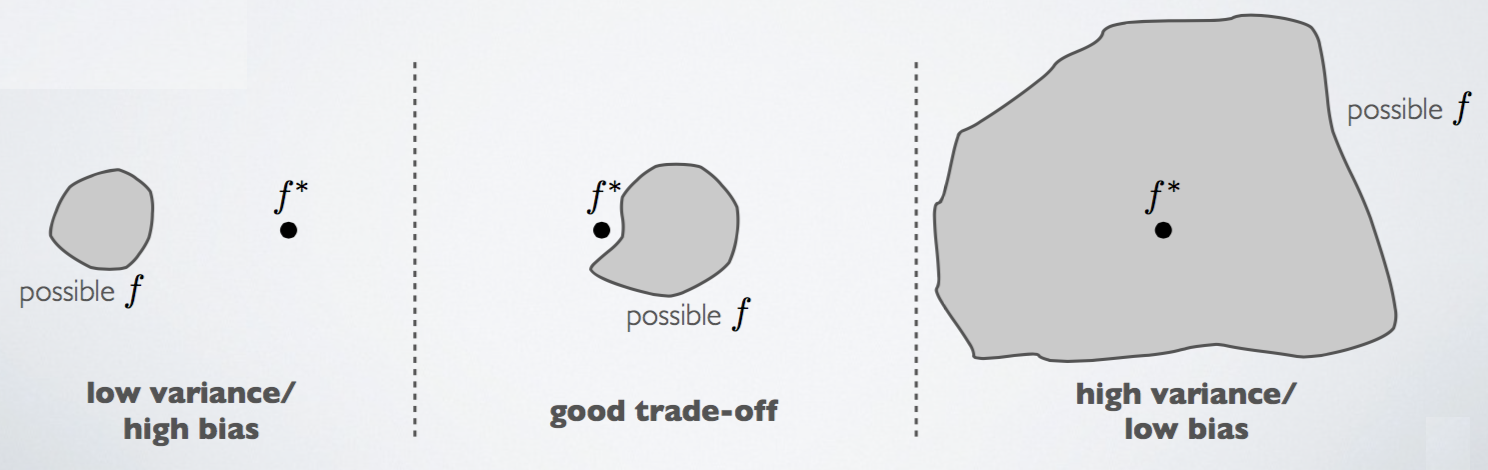
There is a bias-variance trade-off, in which improvement of one is typically at the detriment of the other.
You can think of generalization error as the sum of bias and variance. You want to keep both low, if possible.
Overfitting can happen if your hypothesis is too complex, which can happen if you have too many features. So you will want to through a feature selection phase and pick out features which seem to provide the most value.
Alternatively, you can use the technique of regularization, in which you keep all your features, but reduce the magnitudes/values of parameters
Regularization can be defined as any method which aims to reduce the generalization error of a model though it may not have the same effect on the training error. Since good generalization error is the main goal of machine learning, regularization is essential to success.
Perhaps the most common form of regularization aims to favor smaller parameters. The intuition is that, if you have small values for your parameters
In practice, there may be many combination of parameters which fit your data well. However, some may overfit/not generalize well. We want to introduce some means of valuing these simpler hypotheses over more complex ones (i.e. with larger parameters). We can do so with regularization.
So generally regularization is about shrinking your parameters to make them smaller; for this reason it is sometimes called weight decay. For linear regression, you accomplish this by modifying the cost function to include the term
Note that we are not shrinking
The additional
A regularization method used in linear regression; the L2 norm of the parameters is constrained so that it less than or equal to some specified value (that is, this is L2 regularization):
Where:
LASSO (Least Absolute Shrinkage and Selection Operator) is a regularization method which constrains the L1 norm of the parameters such that it is less than or equal to some specified value:
(These two regularization methods are sometimes called shrinkage methods)
We can update gradient descent to work with our regularization term:
The
If we are using the normal equation, we can update it to a regularized form as well:
Where
We can also update the logistic regression cost function with the regularization term:
Then we can update gradient descent with the new derivative of this cost function for the parameters
It looks the same as the one for linear regression, but again, the actual hypothesis function
Fundamentally, machine learning is all about data:
So there is a lot of uncertainty - we can use probability theory to express this uncertainty in the form of probabilistic models. Generally, learning probabilistic models is known as probablistic machine learning; here we are primarily concerned with non-Bayesian machine learning.
We have some data
We have a parameter
A probabilistic model is just a parameterized joint distribution over all the variables:
We usually interpret such models as a generative model - how was our observed data generated by the world?
So the problem of inference is about learning about our latent variables given the observed data, which we can get via the posterior distribution:
Learning is typically posed as a maximum likelihood problem; that is, we try to find
Then, to make a prediction we want to compute the conditional distribution of some future data:
Or, for classification, if we some classes, each parameterizing a joint distribution, we want to pick the class which maximizes the probability of the observed data:
Discriminative learning algorithms include algorithms like logistic regression, decision trees, kNN, and SVM. Discriminative approaches try to find some way of separating data (discriminating them), such as in logistic regression which tries to find a dividing line and then sees where new data lies in relation to that line. They are unconcerned with how the data was generated.
Say our input features are
Discriminative learning algorithms learn
Generative learning algorithms instead tries to develop a model for each class and sees which model new data conforms to.
Generative learning algorithms learn
It is easier to estimate the conditional distribution
For both discriminative and generative approaches, you will have parameters and latent variables
Say we have some observed values
If we flip this we get the likelihood of
Likelihood is just the name for the probability of observed data as a function of the parameters.
The maximum likelihood estimation is the
(The Expectation-Maximization (EM) algorithm is a way of computing a maximum likelihood estimate for situations where some variables may be hidden.)
If the random variables associated with the values, i.e.
Sometimes this is just notated
So we are looking to estimate the
Logarithms are used, however, for convenience (i.e. dealing with sums rather than products), so instead we are often maximizing the log likelihood (which has its maximum at the same value (i.e. the same argmax) as the regular likelihood, though the actual maximum value may be different):
Another way of explaining MLE:
We have some data
(Notation note:
Though the logarithm version mentioned above is typically preferred to avoid underflow.
Typically, we are more interested in the conditional probability
Assuming the examples are iid, this is:
Say we have a coin which may be unfair. We flip it ten times and get HHHHTTTTTT (we'll call this observed data
Here we just have a binomial distribution so the parameters here are
Where
For this case our MLE would be
Also formulated as:
For a Gaussian distribution, the sample mean is the MLE.
The expectation maximization (EM) algorithm is a two-staged iterative algorithm.
Say you have a dataset which is missing some values. How can you complete your data?
The EM algorithm allows you to do so.
The two stages work as such:
Intuitively, what EM does is tries to find the parameters
Say we have two coins
We conduct 5 experiments in which we randomly choose one of the coins (with equal probability) and flip it 10 times.
We have the following results:
1. HTTTHHTHTH
2. HHHHTHHHHH
3. HTHHHHHTHH
4. HTHTTTHHTT
5. THHHTHHHTH
We are still interested in learning a parameter for each coin,
If we knew which coin we flipped during each experiment, this would be a simple MLE problem. Say we did know which coin was picked for each experiment:
1. B: HTTTHHTHTH
2. A: HHHHTHHHHH
3. A: HTHHHHHTHH
4. B: HTHTTTHHTT
5. A: THHHTHHHTH
Then we just use MLE and get:
That is, for each coin we just compute
But, alas, we are missing the data of which coin we picked for each experiment. We can instead apply the EM algorithm.
Say we initially guess that
We're dealing with a binomial distribution here, so we are using:
The binomial coefficient is the same for both coins (the
For the first experiment we have 5 heads (and
So for this first iteration and for the first experiment, we estimate that the chance of the picked coin being coin
Then we generate the weighted set of these possible completions by computing how much each of these coins, as weighted by the probabilities we just computed, contributed to the results for this experiment (
Then we repeat this for the rest of the experiments, getting the following weighted values for each coin for each experiment:
and sum up the weighted values for each coin:
Then we use these weighted values and MLE to update
And repeat until convergence.
In K-Means we make hard assignments of datapoints to clusters (that is, they belong to only one cluster at a time, and that assignment is binary).
EM is similar to K-Means, but we use soft assignments instead - datapoints can belong to multiple clusters in varying strengths (the "strengths" are probabilities of assignment to each cluster). When the centroids are updated, they are updated against all points, weighted by assignment strength (whereas in K-Means, centroids are updated only against their members).
EM converges to approximately the same clusters as K-Means, except datapoints still have some membership to other clusters (though they may be very weak memberships).
In EM, we consider that each datapoint is generated from a mixture of classes.
For each
These terms may be notated:
What this is modeling here is that each centroid is the center of a Gaussian distribution, and we try to fit these centroids and their distributions to the data.